In my last post, we learned about qubits, superposition, and basic quantum gates. Today, we’re exploring entanglement. This is the phenomenon that makes quantum computing fundamentally different from classical computing.
You’ve probably heard entanglement described as spooky or weird. But what does it actually mean for your code? Let me show you through examples.
What Problem Are We Trying to Solve?
Imagine you need to generate two random numbers that are perfectly correlated:
- Each number is random (50% chance of 0, 50% chance of 1)
- But if the first is 0, the second is always 0
- If the first is 1, the second is always 1
- You don’t know what they’ll be until you check
Let’s try this classically first, then see how quantum entanglement does it differently.
The Classical Approach: Pre-Determined Values
Here’s the obvious classical solution:
import random

class CorrelatedPair:
    def __init__(self):
        # Generate a random value and store it
        self.value = random.choice([0, 1])

    def get_first(self):
        return self.value

    def get_second(self):
        return self.value

# Test it
pair = CorrelatedPair()
print(f"First:  {pair.get_first()}")
print(f"Second: {pair.get_second()}")

# Run multiple trials
print("\n10 trials:")
for i in range(10):
    pair = CorrelatedPair()
    first = pair.get_first()
    second = pair.get_second()
    print(f"Trial {i+1}: first={first}, second={second}, match={first==second}")
Output:
First:  0
Second: 0

10 trials:
Trial 1: first=0, second=0, match=True
Trial 2: first=0, second=0, match=True
Trial 3: first=0, second=0, match=True
Trial 4: first=1, second=1, match=True
Trial 5: first=1, second=1, match=True
Trial 6: first=1, second=1, match=True
Trial 7: first=0, second=0, match=True
Trial 8: first=0, second=0, match=True
Trial 9: first=0, second=0, match=True
Trial 10: first=0, second=0, match=True
Perfect! 100% correlation. The secret? We stored the value when we created the pair.
The Classical Limitation
This classical approach works, but notice what’s happening:
- The value exists before we read it (stored in
self.value) - It’s predetermined when we call
__init__() - Reading it doesn’t change anything
This seems obvious, right? How else could it work?
Now watch what quantum entanglement does differently.
Quantum Entanglement: True Randomness with Perfect Correlation
Let’s create the quantum version using Qiskit.
Setup
from qiskit import QuantumCircuit
from qiskit_aer import AerSimulator

simulator = AerSimulator()
Creating Entangled Qubits
Here’s how to create two entangled qubits:
# Create a circuit with 2 qubits and 2 classical bits
qc = QuantumCircuit(2, 2)

# Step 1: Create superposition on first qubit
qc.h(0)

# Step 2: Entangle the qubits with CNOT
qc.cx(0, 1)

# Step 3: Measure both qubits
qc.measure(0, 0)
qc.measure(1, 1)

print(qc.draw())
Output:
     ┌───┐     ┌─┐
q_0: ┤ H ├──■──┤M├───
     └───┘┌─┴─┐└╥┘┌─┐
q_1: ─────┤ X ├─╫─┤M├
          └───┘ ║ └╥┘
c: 2/═══════════╩══╩═
                0  1
Let me explain what’s happening:
- H gate on q_0: Creates superposition: $\frac{1}{\sqrt{2}}(|0\rangle + |1\rangle)$
- CNOT gate (cx): Links q_1 to q_0. This is the key to entanglement.
- Measure: Now both qubits collapse to definite values
The resulting state is called a Bell state:
$$|\Phi^+\rangle = \frac{1}{\sqrt{2}}(|00\rangle + |11\rangle)$$Translation: 50% chance of both being 0, and 50% chance of both being 1. Never 01 or 10.
Running the Entangled Circuit
job = simulator.run(qc, shots=1000)
result = job.result()
counts = result.get_counts()

print(counts)
Output:
{'00': 509, '11': 491}
Notice anything? We only get 00 or 11. Never 01 or 10.
The qubits are perfectly correlated, just like our classical example!
So What’s the Difference?
Here’s the key difference that took me weeks to understand:
Classical: Value Exists Before Measurement
pair = CorrelatedPair()
# At this point, pair.value already exists (let's say it's 1)
# We just haven't looked at it yet

first = pair.get_first()   # Returns 1 (was already 1)
second = pair.get_second() # Returns 1 (was already 1)
Quantum: Value Doesn’t Exist Until Measurement
# Create entangled qubits
qc = QuantumCircuit(2, 2)
qc.h(0)
qc.cx(0, 1)
# At this point, NEITHER qubit has a definite value
# They're in superposition: (|00⟩ + |11⟩)/√2

qc.measure(0, 0)  # NOW q_0 randomly becomes 0 or 1
qc.measure(1, 1)  # And q_1 INSTANTLY matches it
This might seem like a subtle distinction, but it has huge implications.
Understanding the CNOT Gate
The CNOT (Controlled-NOT) gate is your primary tool for creating entanglement. Let’s understand it properly.
CNOT has two qubits:
- Control qubit: The boss
- Target qubit: Gets flipped IF control is in state 1
Here’s the truth table:
| Control | Target | After CNOT |
|---|---|---|
| 0 | 0 | 00 |
| 0 | 1 | 01 |
| 1 | 0 | 11 (target flipped!) |
| 1 | 1 | 10 (target flipped!) |
Let’s see it in code:
# Case 1: Control=0, Target=0 → Result: 00
qc1 = QuantumCircuit(2, 2)
qc1.cx(0, 1)  # Both start at |0⟩
qc1.measure([0, 1], [0, 1])

# Case 2: Control=1, Target=0 → Result: 11
qc2 = QuantumCircuit(2, 2)
qc2.x(0)      # Set control to |1⟩
qc2.cx(0, 1)  # Target flips from 0 to 1
qc2.measure([0, 1], [0, 1])

# Case 3: Control=0, Target=1 → Result: 01
qc3 = QuantumCircuit(2, 2)
qc3.x(1)      # Set target to |1⟩
qc3.cx(0, 1)  # Control is 0, so nothing happens
qc3.measure([0, 1], [0, 1])

# Case 4: Control=1, Target=1 → Result: 10
qc4 = QuantumCircuit(2, 2)
qc4.x(0)      # Set control to |1⟩
qc4.x(1)      # Set target to |1⟩
qc4.cx(0, 1)  # Target flips from 1 to 0
qc4.measure([0, 1], [0, 1])

for i, qc in enumerate([qc1, qc2, qc3, qc4], 1):
    counts = simulator.run(qc, shots=100).result().get_counts()
    print(f"Case {i}: {counts}")
Output:
Case 1: {'00': 100}
Case 2: {'11': 100}
Case 3: {'10': 100}
Case 4: {'01': 100}
The magic happens when you combine CNOT with superposition:
qc = QuantumCircuit(2, 2)

# Put control in superposition
qc.h(0)  # Now q_0 is: (|0⟩ + |1⟩)/√2

# Apply CNOT
qc.cx(0, 1)
# If q_0 is |0⟩ component: target stays 0 → |00⟩
# If q_0 is |1⟩ component: target flips to 1 → |11⟩
# Result: (|00⟩ + |11⟩)/√2 ← Entangled!

qc.measure([0, 1], [0, 1])
counts = simulator.run(qc, shots=1000).result().get_counts()
print(counts)
# Output: {'00': ~500, '11': ~500}
The CNOT spreads the superposition from the control to the target, creating entanglement.
Visualizing the Difference
Let me show you why this matters with a simple experiment:
Classical: You Can Peek Without Consequences
class ClassicalPair:
    def __init__(self):
        self.value = random.choice([0, 1])

    def peek(self):
        # Looking doesn't change anything
        return self.value

    def measure(self):
        return self.value

pair = ClassicalPair()
peek1 = pair.peek()
peek2 = pair.peek()
final = pair.measure()

print(f"Peek 1: {peek1}")
print(f"Peek 2: {peek2}")
print(f"Final:  {final}")
# All three are identical because peeking doesn't affect the value
Output:
Peek 1: 1
Peek 2: 1
Final:  1
Quantum: You Cannot Peek
# Try to peek at quantum state
qc = QuantumCircuit(2, 2)
qc.h(0)
qc.cx(0, 1)

# If we measure here...
qc.measure(0, 0)
# The superposition COLLAPSES
# We can't peek without destroying the entanglement

# Any further operations now work on collapsed state, not superposition
This is fundamental: measurement is destructive in quantum computing.
Why This Matters: The Computational Advantage
Now for the practical question: Why should programmers care about entanglement?
Exponential State Space
Here’s the key insight:
Classical: With $n$ bits, you can represent 1 state at a time.
- 3 bits: store one of 8 states (000, 001, 010, 011, 100, 101, 110, 111)
- To process all 8, you need 8 separate computations
Quantum: With $n$ entangled qubits, you can represent all $2^n$ states simultaneously in superposition.
- 3 qubits: process all 8 states at once
- 10 qubits: process 1,024 states at once
- 50 qubits: process 1,125,899,906,842,624 states at once
Let me show you:
# Classical: Process 4 states one at a time
def classical_search(data):
    """Search through data one item at a time"""
    for i, item in enumerate(data):
        # Check if item matches condition
        if item == target:
            return i
    return -1

# Time complexity: O(n) because we check items linearly

# Quantum: Process all states in superposition
def quantum_search_concept():
    """
    With entanglement and superposition:
    1. Put all inputs in superposition (parallel processing)
    2. Apply quantum operations to ALL states simultaneously
    3. Use interference to amplify the correct answer
    4. Measure to get result
    """
    # Time complexity: O(√n) which is a quadratic speedup
    pass
Comparing Time Complexity
| Problem Size | Classical Operations | Quantum Operations (with entanglement) |
|---|---|---|
| 4 items | 4 | 2 |
| 16 items | 16 | 4 |
| 100 items | 100 | 10 |
| 1,000,000 | 1,000,000 | 1,000 |
This is why quantum computers can solve certain problems exponentially faster.
Building Different Entangled States
The Bell state we created is just one type of entanglement. Let’s create others:
Anti-Correlated State
qc = QuantumCircuit(2, 2)

qc.h(0)
qc.cx(0, 1)
qc.x(1)  # Flip the second qubit

qc.measure([0, 1], [0, 1])

counts = simulator.run(qc, shots=1000).result().get_counts()
print("Anti-correlated state:", counts)
Output:
Anti-correlated state: {'01': 521, '10': 479}
Now they’re always opposite! If first is 0, second is 1, and vice versa.
This creates the state: $\frac{1}{\sqrt{2}}(|01\rangle + |10\rangle)$
Three-Qubit Entanglement (GHZ State)
qc = QuantumCircuit(3, 3)

qc.h(0)       # Superposition on first qubit
qc.cx(0, 1)   # Entangle first with second
qc.cx(0, 2)   # Entangle first with third

qc.measure([0, 1, 2], [0, 1, 2])

counts = simulator.run(qc, shots=1000).result().get_counts()
print("GHZ state:", counts)
Output:
GHZ state: {'111': 504, '000': 496}
All three qubits are now correlated! This is the state:
$$|GHZ\rangle = \frac{1}{\sqrt{2}}(|000\rangle + |111\rangle)$$You can entangle as many qubits as you want this way.
Practical Example: Controlled Operations
Entanglement is essential for controlled operations. This is where one qubit controls what happens to others.
def controlled_computation(control_value):
    """
    Perform different operations based on control qubit.
    This is impossible without entanglement!
    """
    qc = QuantumCircuit(3, 3)

    # Set control qubit based on input
    if control_value == 1:
        qc.x(0)

    # Create superposition on working qubits
    qc.h(1)
    qc.h(2)

    # Controlled operations: only execute if control is |1⟩
    qc.cx(0, 1)  # If control=1, flip qubit 1
    qc.cx(0, 2)  # If control=1, flip qubit 2

    qc.measure([0, 1, 2], [0, 1, 2])

    counts = simulator.run(qc, shots=1000).result().get_counts()
    return counts

print("Control = 0:")
print(controlled_computation(0))
# Output: Results will have bit 0 = 0

print("\nControl = 1:")
print(controlled_computation(1))
# Output: Results will have bit 0 = 1, and qubits 1,2 affected
Output:
Control = 0:
{'100': 245, '010': 246, '000': 235, '110': 274}

Control = 1:
{'111': 254, '101': 224, '011': 256, '001': 266}
This pattern appears in many quantum algorithms where you need conditional logic.
Common Misconceptions
Let me address some confusion I had:
Does entanglement allow instant communication?
No! When you measure one qubit, you get a random result. The other person measuring their qubit also gets a random result. The correlation only shows up when you compare results later (through classical communication).
Is entanglement just classical correlation with extra steps?
No! Classical correlation requires predetermined values. Quantum entanglement has no values until measurement. The qubits are genuinely in superposition.
Can I use entanglement to copy quantum states?
No. The no-cloning theorem says you can’t duplicate unknown quantum states. Entanglement creates correlation, not copies.
Testing Your Understanding
Try these exercises:
Exercise 1: Detect Entanglement
Write a function that checks if a circuit produces entangled qubits:
def is_entangled(qc, threshold=0.8):
    """
    Check if a 2-qubit circuit produces entangled state.
    Returns True if measurements show strong correlation.
    """
    job = simulator.run(qc, shots=1000)
    counts = job.result().get_counts()

    # Entangled states show strong correlation
    # Either mostly 00,11 or mostly 01,10
    same = counts.get('00', 0) + counts.get('11', 0)
    opposite = counts.get('01', 0) + counts.get('10', 0)

    max_correlation = max(same, opposite) / 1000
    return max_correlation > threshold

# Test with entangled state
qc_entangled = QuantumCircuit(2, 2)
qc_entangled.h(0)
qc_entangled.cx(0, 1)
qc_entangled.measure([0, 1], [0, 1])

# Test with non-entangled state
qc_separate = QuantumCircuit(2, 2)
qc_separate.h(0)
qc_separate.h(1)
qc_separate.measure([0, 1], [0, 1])

print(f"Entangled: {is_entangled(qc_entangled)}")    # True
print(f"Separate: {is_entangled(qc_separate)}")      # False
Exercise 2: Four-Qubit Entanglement
Can you create a state where all four qubits are entangled?
Hint: Start with H on the first qubit, then use CNOT to spread entanglement.
